Beta-binomial test
Thang V Pham
4 February 2021
Installation
The R package countdata implements the beta-binomial test for comparative analysis of count data.
To install the package
install.packages("countdata")Two-group comparison
Load the ion library and load an example dataset (or pointing to your local, tab-delimitated data file)
source("https://tvpham.github.io/ion.r")

d <- ion$load("https://tvpham.github.io/data/example-3groups.txt")
Check the head of the loaded data
head(d)## a1 a2 a3 b1 b2 b3 c1 c2
## 1 624 496 509 414 394 375 325 288
## 2 615 854 930 341 523 360 359 329
## 3 553 560 745 819 490 481 480 500
## 4 525 412 401 354 321 310 258 228
## 5 484 284 315 268 282 307 270 298
## 6 482 348 400 242 365 367 81 118Suppose that there are three groups a, b and c as indicated by the column names. To compare the a samples to the b samples and store the result, call
out <- ion$beta_binomial_2g(d,
                            c("a1", "a2", "a3"),
                            c("b1", "b2", "b3"))

ion$save(out, "output.txt")
In the first statement, the first parameter is the raw count data. The second parameter is the column names of the first group and the third parameter the column names of the second group. The returned value out is a list of three components “fc” fold change, “pval” p-value, and “pval.BH” p-value adjusted for multiple testing using the Benjamini-Hochberg method (Benjamini & Hochberg, 1995).
The second statement saves the returned value to a tab-deliminated text file. Examine the content of output.txt.
We often want to write out the normalized count data as well. This is because the beta-binomial test uses the normalized values internally. The normalized values are obtained by scaling the original count values so that the total counts are equal across all samples.
d_norm <- ion$normalize_global(d)

ion$save(cbind(d, d_norm, out), "output.txt")
Here we use the R function cbind to combine tables/lists with the same number of rows into one. After normalization, the total counts should be identical.
colSums(d_norm)## a1 a2 a3 b1 b2 b3 c1 c2
## 19159 19159 19159 19159 19159 19159 19159 19159The normalized data d_norm can be used in subsequent analyses, for example for data clustering.
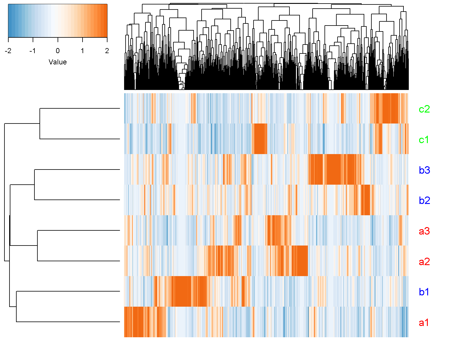
For unsupervised clustering, we do not use the result of any differential analysis
ion$heatmap(t(d_norm),
            z_transform = "col",
            row_labels = colnames(d_norm),
            row_label_colors = c("red", "red", "red", "blue", "blue",
                                 "blue","green", "green"),
            row_margin = 5)
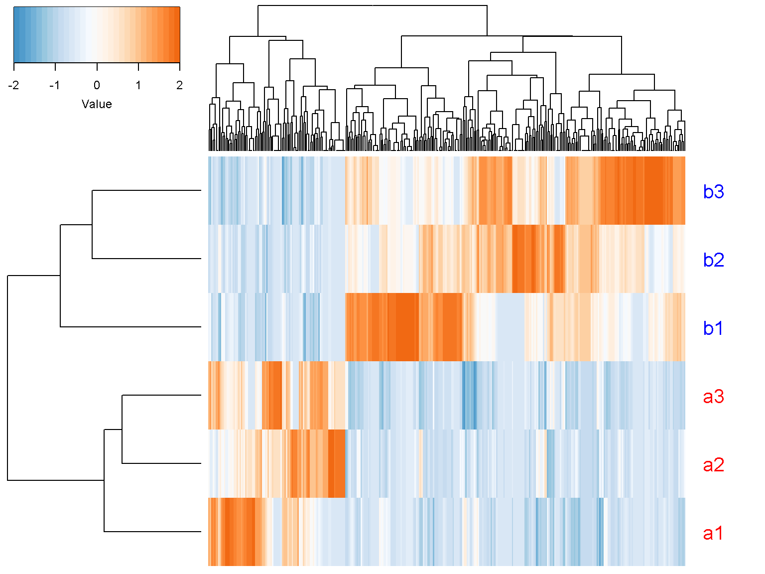
For supervised clustering, we use the data rows with p-value < 0.05.
ion$heatmap(t(d_norm[out$pval < 0.05,
                     c("a1", "a2", "a3", "b1", "b2", "b3")]),
            z_transform = "col",
            row_labels = c("a1", "a2", "a3", "b1", "b2", "b3"),
            row_label_colors = c("red", "red", "red", "blue", "blue", "blue"),
            row_margin = 5)
Three-group comparison
To compare the a, b, and c samples, use the function ion$beta_binomial_3g.
out <- ion$beta_binomial_3g(d,
                            c("a1", "a2", "a3"),
                            c("b1", "b2", "b3"),
                            c("c1", "c2"))
The returned value out contains only two components “pval” and “pval.BH” because there is no fold change among three groups.
There is also a function for a four-group comparison ion$beta_binomial_4g. Refer to the manual for comparison of more than four groups.
Paired sample test
If a and b samples are matched, for example from individual patients before and after treatment, a paired sample test is appropriate
out <- ion$beta_binomial_2g_paired(d,
                                   c("a1", "a2", "a3"),
                                   c("b1", "b2", "b3"))
Note that the sample orders are important so that “a1” is matched to “b1”, “a2” to “b2”, and “a3” to “b3”. The returned value is a list with three components “fc”, “pval”, and “pval.BH” standing for fold change, p-value and corrected p-value, respectively.
Citations
For the independent sample test
Pham TV, Piersma SR, Warmoes M, Jimenez CR (2010) On the beta binomial model for analysis of spectral count data in label-free tandem mass spectrometry-based proteomics. Bioinformatics, 26(3):363-369.
For the paired sample test
Pham TV, Jimenez CR (2012) An accurate paired sample test for count data. Bioinformatics, 28(18):i596-i602.
For the Benjamini-Hochberg method for multiple test correction
Benjamini Y, Hochberg Y (1995) Controlling the false discovery rate: a practical and powerful approach to multiple testing. Journal of the Royal Statistical Society Series B; 57, 289-300.